The goal of cyclingtools is to provide tools for making easier to analyze data in cycling.
Installation
You can install the development version of cyclingtools from GitHub with:
# install.packages("remotes")
remotes::install_github("fmmattioni/cyclingtools")
Usage
Critical Power
Demo data
The package comes with a demonstration data frame to show how the functions work and also to show you how you can setup your data:
library(cyclingtools)

demo_critical_power
#>    PO  TTE
#> 1 446  100
#> 2 385  172
#> 3 324  434
#> 4 290  857
#> 5 280 1361
Simple analysis
Perform a simple analysis from the chosen critical power models:
simple_results <- critical_power(
  .data = demo_critical_power,
  power_output_column = "PO",
  time_to_exhaustion_column = "TTE",
  method = c("3-hyp", "2-hyp", "linear", "1/time"),
  plot = TRUE,
  all_combinations = FALSE,
  reverse_y_axis = FALSE
)

simple_results
#> # A tibble: 4 x 12
#>   method data  model    CP `CP SEE`   `W'` `W' SEE`  Pmax `Pmax SEE`    R2
#>   <chr>  <lis> <lis> <dbl>    <dbl>  <dbl>    <dbl> <dbl>      <dbl> <dbl>
#> 1 3-hyp  <tib… <nls>  260.      3.1 27410.    4794  1004.       835. 0.998
#> 2 2-hyp  <tib… <nls>  262.      1.6 24174.    1889.   NA         NA  0.997
#> 3 linear <tib… <lm>   266.      3   20961.    2248.   NA         NA  1.00
#> 4 1/time <tib… <lm>   274.      6.2 17784.    1160    NA         NA  0.987
#> # … with 2 more variables: RMSE <dbl>, plot <list>
You can also plot the results:
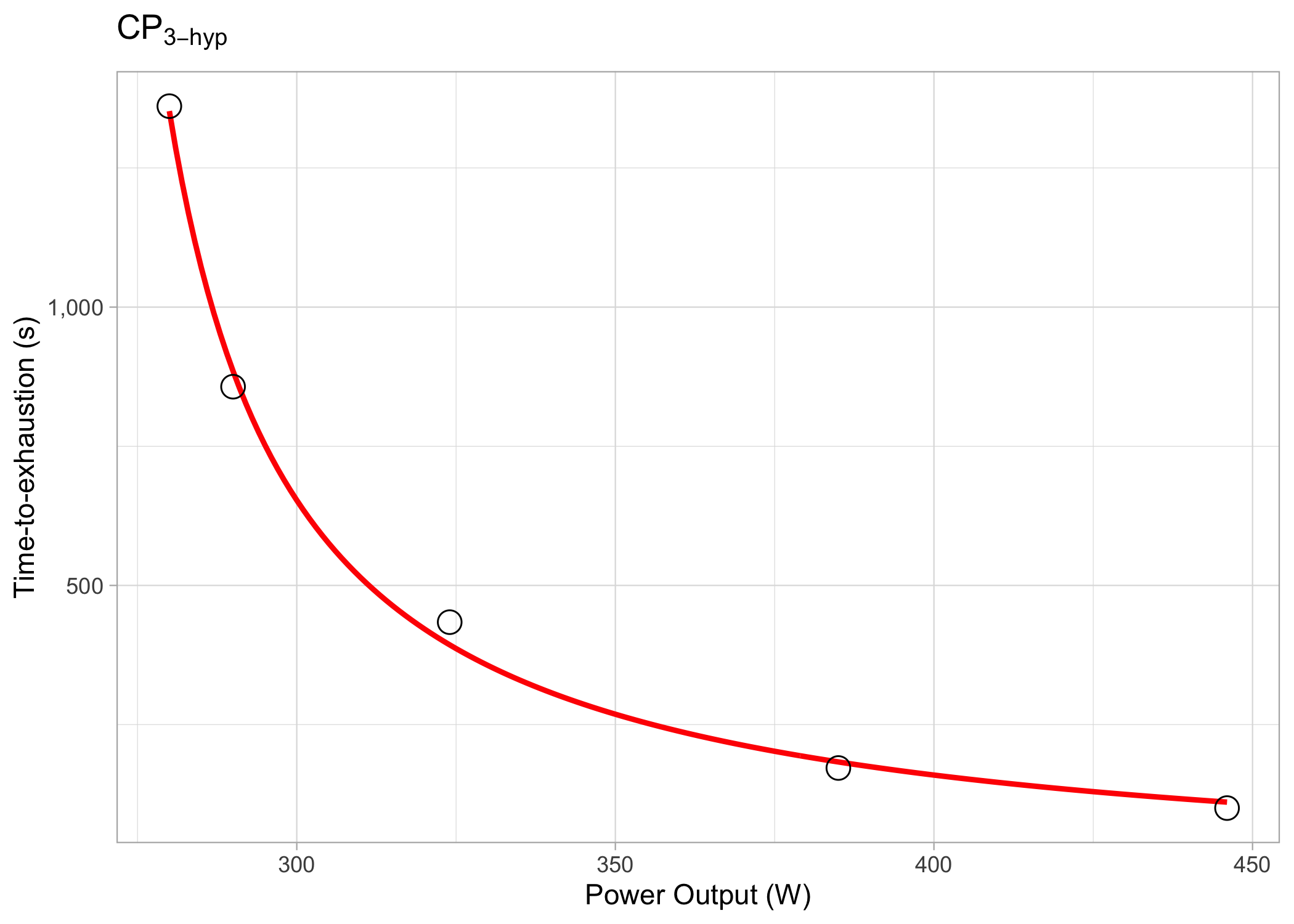
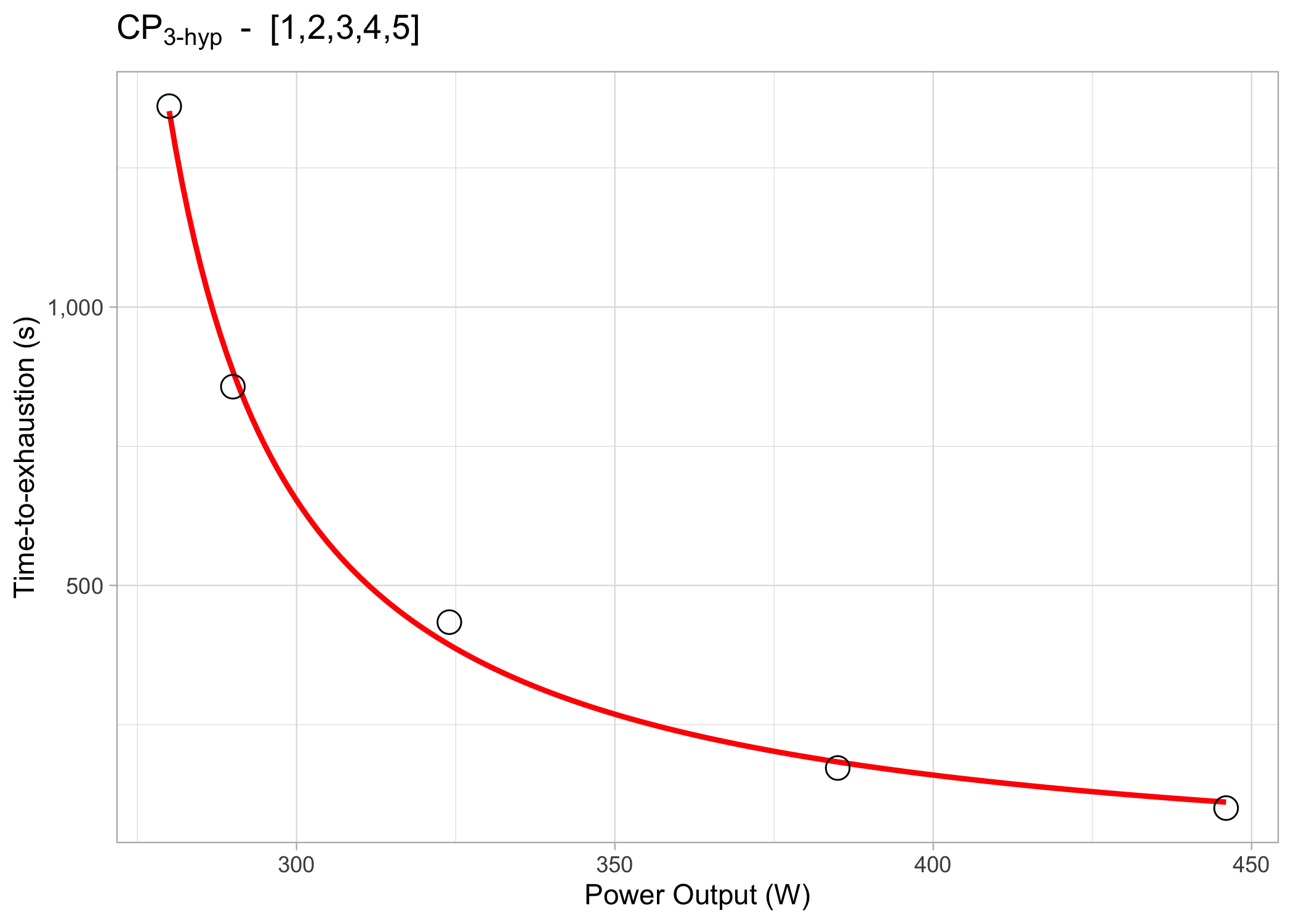
All possible combinations analysis
You can also perform an analysis with all the possible combinations of time-to-exhaustion trials provided. All you need to do is to set all_combinations = TRUE:
combinations_results <- critical_power(
  .data = demo_critical_power,
  power_output_column = "PO",
  time_to_exhaustion_column = "TTE",
  method = c("3-hyp", "2-hyp", "linear", "1/time"),
  plot = TRUE,
  all_combinations = TRUE,
  reverse_y_axis = FALSE
)

combinations_results
#> # A tibble: 74 x 13
#>    index method data  model    CP `CP SEE`   `W'` `W' SEE`  Pmax `Pmax SEE`
#>    <chr> <chr>  <lis> <lis> <dbl>    <dbl>  <dbl>    <dbl> <dbl>      <dbl>
#>  1 [1,2… 3-hyp  <tib… <nls>  260.      3.1 27410.    4794  1004.      835.
#>  2 [1,2… 2-hyp  <tib… <nls>  262.      1.6 24174.    1889.   NA        NA
#>  3 [1,2… linear <tib… <lm>   266.      3   20961.    2248.   NA        NA
#>  4 [1,2… 1/time <tib… <lm>   274.      6.2 17784.    1160    NA        NA
#>  5 [1,2… 3-hyp  <tib… <nls>  246.      6.2 42699.    7655   595.       70.2
#>  6 [1,2… 2-hyp  <tib… <nls>  261.      4.7 24814.    3691.   NA        NA
#>  7 [1,2… linear <tib… <lm>   269.      5.9 19977.    2877.   NA        NA
#>  8 [1,2… 1/time <tib… <lm>   278.      7.9 17194.    1339.   NA        NA
#>  9 [1,2… 3-hyp  <tib… <nls>  255       1.9 36462.    3328.  627.       63.7
#> 10 [1,2… 2-hyp  <tib… <nls>  262.      2.2 24940.    2882.   NA        NA
#> # … with 64 more rows, and 3 more variables: R2 <dbl>, RMSE <dbl>, plot <list>
You can also plot the results:
Critical Speed
Demo data
demo_critical_speed
#> # A tibble: 3 x 2
#>   Distance   TTE
#>      <int> <int>
#> 1      956   180
#> 2     1500   300
#> 3     3399   720
Simple analysis
Perform a simple analysis from the chosen critical power models:
simple_results <- critical_speed(
  .data = demo_critical_speed,
  distance_column = "Distance",
  time_to_exhaustion_column = "TTE",
  method = c("3-hyp", "2-hyp", "linear", "1/time"),
  plot = TRUE,
  all_combinations = FALSE,
  reverse_y_axis = FALSE
)

simple_results
#> # A tibble: 3 x 10
#>   method data             model     CS `CS SEE`  `D'` `D' SEE`    R2  RMSE plot
#>   <chr>  <list>           <list> <dbl>    <dbl> <dbl>    <dbl> <dbl> <dbl> <lis>
#> 1 2-hyp  <tibble [3 × 3]> <nls>   4.52        0  143.     0.94  1.00  1.43 <gg>
#> 2 linear <tibble [3 × 3]> <lm>    4.52        0  142.     1     1     0.86 <gg>
#> 3 1/time <tibble [3 × 3]> <lm> 4.53 0 142. 1.02 1.00 0 <gg>Coming soon
Training impulse analyses (iTRIMP, bTRIMP, eTRIMP, luTRIMP)
Suggestions? Feel free to open an issue!
Related work
cycleRtools: A suite of functions for analysing cycling data.
Citation
citation("cyclingtools")
#>
#> Maturana M, Felipe, Fontana, Y F, Pogliaghi, Silvia, Passfield, Louis,
#> Murias, M J (2018). "Critical power: How different protocols and models
#> affect its determination." _Journal of Science and Medicine in Sport_,
#> *21*(7), 1489. doi: 10.1016/j.jsams.2017.11.015 (URL:
#> https://doi.org/10.1016/j.jsams.2017.11.015).
#>
#> A BibTeX entry for LaTeX users is
#>
#>   @Article{,
#>     title = {Critical power: How different protocols and models affect its determination},
#>     author = {Mattioni Maturana and {Felipe} and {Fontana} and Federico Y and {Pogliaghi} and {Silvia} and {Passfield} and {Louis} and {Murias} and Juan M},
#>     journal = {Journal of Science and Medicine in Sport},
#>     volume = {21},
#>     number = {7},
#>     pages = {1489},
#>     year = {2018},
#>     publisher = {Elsevier},
#>     doi = {10.1016/j.jsams.2017.11.015},
#>   }