cyclingtools
cyclingtools.Rmd
Please, note that currently cyclingtools only provide critical power analyses. However, more functionality is planned, such as training impulse analyses (iTRIMP, bTRIMP, eTRIMP, luTRIMP).
If you have a suggestion, feel free to open an issue.
Critical Power analysis
For performing critical power analysis, the general critical_power() function was created. There are basically two main options in there: you can choose which model to fit (i.e., CP 3-hyp, CP 2-hyp, CP linear, and CP 1/time), and you can also choose whether to produce an analysis with all the combinations of the time-to-exhaustion trials provided.
Let’s look at the main functionality:
library(cyclingtools)

simple_results <- critical_power(
  .data = demo_critical_power,
  power_output_column = "PO",
  time_to_exhaustion_column = "TTE",
  method = c("3-hyp", "2-hyp", "linear", "1/time"),
  plot = TRUE,
  all_combinations = FALSE,
  reverse_y_axis = FALSE
)

simple_results
#> # A tibble: 4 × 12
#>   method data     model     CP `CP SEE`   `W'` `W' SEE`  Pmax `Pmax SEE`    R2
#>   <chr>  <list>   <list> <dbl>    <dbl>  <dbl>    <dbl> <dbl>      <dbl> <dbl>
#> 1 3-hyp  <tibble> <nls>   260.      3.1 27410.    4794  1004.       835. 0.998
#> 2 2-hyp  <tibble> <nls>   262.      1.6 24174.    1889.   NA         NA  0.997
#> 3 linear <tibble> <lm>    266.      3   20961.    2248.   NA         NA  1.00
#> 4 1/time <tibble> <lm>    274.      6.2 17784.    1160    NA         NA  0.987
#> # … with 2 more variables: RMSE <dbl>, plot <list>
In the above example, we chose to fit critical power on all the available methods, but you can also just choose one or two:
critical_power(
  .data = demo_critical_power,
  power_output_column = "PO",
  time_to_exhaustion_column = "TTE",
  method = c("3-hyp", "2-hyp"),
  plot = TRUE,
  all_combinations = FALSE,
  reverse_y_axis = FALSE
)
#> # A tibble: 2 × 12
#>   method data     model     CP `CP SEE`   `W'` `W' SEE`  Pmax `Pmax SEE`    R2
#>   <chr>  <list>   <list> <dbl>    <dbl>  <dbl>    <dbl> <dbl>      <dbl> <dbl>
#> 1 3-hyp  <tibble> <nls>   260.      3.1 27410.    4794  1004.       835. 0.998
#> 2 2-hyp  <tibble> <nls>   262.      1.6 24174.    1889.   NA         NA  0.997
#> # … with 2 more variables: RMSE <dbl>, plot <list>
The nice thing about the retrieved results is that the model is saved as well. So you can further explore it if you would like to. For example, using the base R function summary():
simple_results %>%
  dplyr::slice(1) %>%
  dplyr::pull(model) %>%
  .[[1]] %>%
  summary()
#>
#> Formula: TTE ~ (AWC/(PO - CP)) + (AWC/(CP - Pmax))
#>
#> Parameters:
#>       Estimate Std. Error t value Pr(>|t|)
#> AWC  27409.928   4794.045   5.717 0.029255 *
#> CP     260.267      3.097  84.038 0.000142 ***
#> Pmax  1003.832    834.676   1.203 0.352171
#> ---
#> Signif. codes:  0 '***' 0.001 '**' 0.01 '*' 0.05 '.' 0.1 ' ' 1
#>
#> Residual standard error: 37.14 on 2 degrees of freedom
#>
#> Number of iterations to convergence: 5
#> Achieved convergence tolerance: 1.49e-08
Or the broom::tidy() function:
simple_results %>%
  dplyr::slice(1) %>%
  dplyr::pull(model) %>%
  .[[1]] %>%
  broom::tidy()
#> # A tibble: 3 × 5
#>   term  estimate std.error statistic  p.value
#>   <chr>    <dbl>     <dbl>     <dbl>    <dbl>
#> 1 AWC     27410.   4794.        5.72 0.0293
#> 2 CP        260.      3.10     84.0  0.000142
#> 3 Pmax     1004.    835.        1.20 0.352
The above can also be more quickly achieved with the following:
simple_results %>%
  dplyr::select(method, model) %>%
  dplyr::rowwise() %>%
  dplyr::mutate(tidy_model = broom::tidy(model) %>% list()) %>%
  tidyr::unnest(cols = tidy_model)
#> # A tibble: 9 × 7
#>   method model  term        estimate std.error statistic     p.value
#>   <chr>  <list> <chr>          <dbl>     <dbl>     <dbl>       <dbl>
#> 1 3-hyp  <nls>  AWC           27410.   4794.        5.72 0.0293
#> 2 3-hyp  <nls>  CP              260.      3.10     84.0  0.000142
#> 3 3-hyp  <nls>  Pmax           1004.    835.        1.20 0.352
#> 4 2-hyp  <nls>  AWC           24175.   1889.       12.8  0.00103
#> 5 2-hyp  <nls>  CP              262.      1.58    166.   0.000000485
#> 6 linear <lm>   (Intercept)   20961.   2248.        9.32 0.00261
#> 7 linear <lm>   TTE             265.      3.00     88.6  0.00000317
#> 8 1/time <lm>   (Intercept)     274.      6.16     44.4  0.0000251
#> 9 1/time <lm>   I(1/TTE)      17784.   1160.       15.3  0.000603
Multiple combinations
The all_combinations argument let you decide whether to perform multiple fits from all the possible combinations of trials provided:
combinations_results <- critical_power(
.data = demo_critical_power,
power_output_column = "PO",
time_to_exhaustion_column = "TTE",
method = c("3-hyp", "2-hyp", "linear", "1/time"),
plot = TRUE,
all_combinations = TRUE,
reverse_y_axis = FALSE
)
combinations_results
#> # A tibble: 74 × 13
#> index method data model CP `CP SEE` `W'` `W' SEE` Pmax `Pmax SEE`
#> <chr> <chr> <list> <lis> <dbl> <dbl> <dbl> <dbl> <dbl> <dbl>
#> 1 [1,2,3… 3-hyp <tibble> <nls> 260. 3.1 27410. 4794 1004. 835.
#> 2 [1,2,3… 2-hyp <tibble> <nls> 262. 1.6 24174. 1889. NA NA
#> 3 [1,2,3… linear <tibble> <lm> 266. 3 20961. 2248. NA NA
#> 4 [1,2,3… 1/time <tibble> <lm> 274. 6.2 17784. 1160 NA NA
#> 5 [1,2,3… 3-hyp <tibble> <nls> 246. 6.2 42699. 7655 595. 70.2
#> 6 [1,2,3… 2-hyp <tibble> <nls> 261. 4.7 24814. 3691. NA NA
#> 7 [1,2,3… linear <tibble> <lm> 269. 5.9 19977. 2877. NA NA
#> 8 [1,2,3… 1/time <tibble> <lm> 278. 7.9 17194. 1339. NA NA
#> 9 [1,2,3… 3-hyp <tibble> <nls> 255 1.9 36462. 3328. 627. 63.7
#> 10 [1,2,3… 2-hyp <tibble> <nls> 262. 2.2 24940. 2882. NA NA
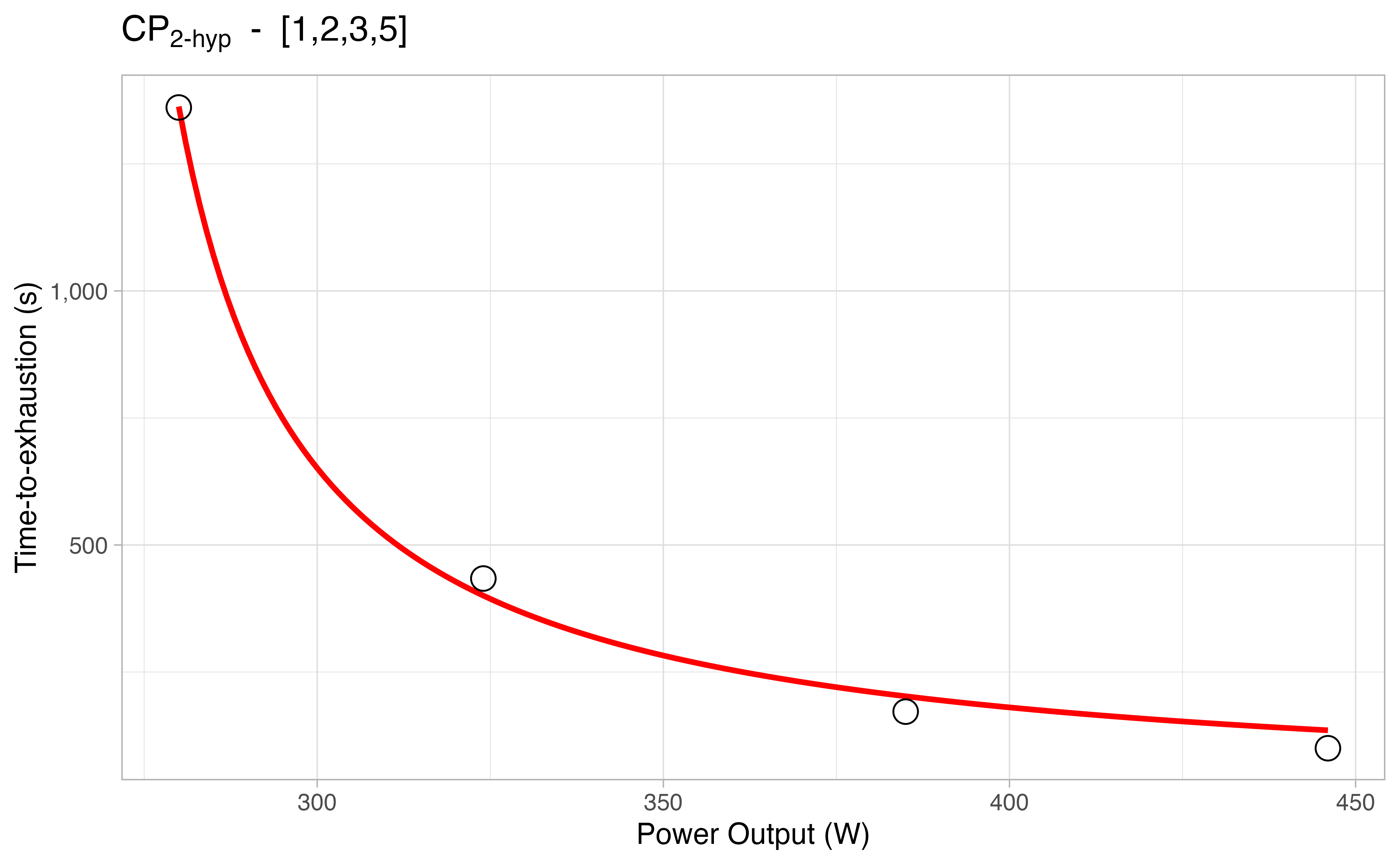
#> # … with 64 more rows, and 3 more variables: R2 <dbl>, RMSE <dbl>, plot <list>You can also check the plots of each estimation in case you set plot = TRUE:
Shiny app
All of these functions can be performed in Critical Power Dashboard