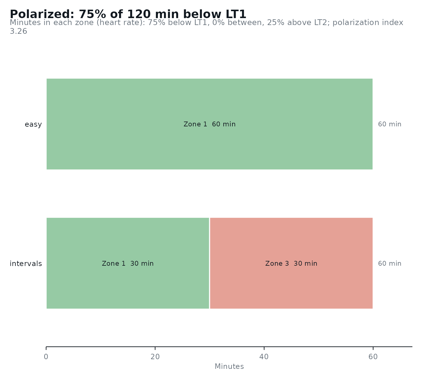
Training load and intensity distribution from the lactate zones

Sorts the samples of training sessions (heart rate, or power or speed) into the zones of lactate_zones(), and returns the time in each zone and the training intensity distribution with its polarization index. It prints a short summary and can be plotted with autoplot().

Usage

training_load(
  data,
  zones,
  column = measure,
  measure = c("heart_rate", "intensity"),
  interval = 1,
  .by = NULL
)

# S3 method for class 'lactate_load'
autoplot(object, ...)

Arguments

data: A data frame with one row per sample, or a numeric vector of samples.
zones: The result of lactate_zones(), with three or five zones.
column: The column of data with the samples. Defaults to the name of measure.
measure: What the samples are: "heart_rate" (bpm; uses the heart rate at the zone boundaries) or "intensity" (power or speed in the unit of the test).
interval: The time between two samples, in seconds. Defaults to 1.
.by: Names of columns that group the samples (e.g. "session" or "week"), kept in the order they appear.
object: The result of training_load().
...: Not used.

Value

a lactate_load tibble with one row per group: minutes, the minutes in each zone (zone_1, ...), the percentage of time in each zone (zone_1_percent, ...), with five zones the percentage in each domain (moderate_percent, heavy_percent, severe_percent), polarization_index, and distribution.

Details

Time in zone: every sample counts for interval seconds in the zone of its value. Missing samples are left out. Heart rate lags behind intensity in short intervals, so heart-rate time in zone under-counts the highest zones in interval sessions; power or speed samples avoid that (Seiler, 2010).
Intensity distribution across the three domains (moderate below LT1, heavy from LT1 to LT2, severe above LT2; with five zones, zones 1-2 and 4-5 are added up). The polarization index is log10((moderate / heavy) * severe * 100), with each domain as a fraction of the total time; when the heavy domain is empty it is set to 0.01 and 0.01 is taken from the severe domain; it is 0 when the severe domain is empty, and not computed (NA) when the severe domain exceeds the moderate one. A distribution is "polarized" when the index is above 2.00 and moderate > severe > heavy (Treff et al., 2019). Otherwise it is labeled "pyramidal" (moderate > heavy > severe), "threshold" (heavy largest), "high intensity" (severe largest), or "other". Treff et al. (2019) note that a threshold distribution can also be pyramidal.

The distribution describes a training period, so give it the samples of all the sessions of that period (e.g. .by = "week").

References

Seiler S. What is best practice for training intensity and duration distribution in endurance athletes? International Journal of Sports Physiology and Performance. 2010;5(3):276-291.

Treff G, Winkert K, Sareban M, Steinacker JM, Sperlich B. The polarization-index: a simple calculation to distinguish polarized from non-polarized training intensity distributions. Frontiers in Physiology. 2019;10:707.

Examples

results <- lactate_threshold(demo_data, intensity, lactate, heart_rate, plot = FALSE)
zones <- lactate_zones(results, lt1 = "Log-log", lt2 = "ModDmax")
## two sessions of heart rate sampled every 5 s
sessions <- data.frame(
  session = rep(c("easy", "intervals"), each = 720),
  heart_rate = c(rep(140, 720), rep(c(150, 185), times = 360))
)
load <- training_load(sessions, zones, interval = 5, .by = "session")
load
#> # Training load: 2 groups, 2.0 h in 3 zones (heart rate)
#> # Distribution:  polarized: 75% moderate, 0% heavy, 25% severe (polarization
#> #   index 3.26)
#>   session   minutes zone_1 zone_2 zone_3 zone_1_percent zone_2_percent
#>   <chr>       <dbl>  <dbl>  <dbl>  <dbl>          <dbl>          <dbl>
#> 1 easy           60     60      0      0            100              0
#> 2 intervals      60     30      0     30             50              0
#> # ℹ 3 more variables: zone_3_percent <dbl>, polarization_index <dbl>,
#> #   distribution <chr>
autoplot(load)