The {metabolic} package provides you all the tools necessary to reproduce the meta-analysis published in Medicine & Science in Sports & Exercise.
You can easily read the paper in the journal website through the function metabolic::read_paper(). It will take you to the online published paper in your default browser.
We also provide you all the data used to perform the meta-analysis and the GOfER (Graphical Overview for Evidence Reviews) diagram. In case you are not familiar with R, or just would like to download the data, you can do so in the metabolic_meta and in the metabolic_gofer vignettes.
Produce an HTML report for a given clinical endpoint
The easiest way of reproducing the meta-analysis for a given clinical endpoint is using the metabolic::build_report()function, which will build an HTML report with all the results, including R output and plots. Try it out! Make sure you also choose a path to save the report to!
library(metabolic)

build_report(endpoint = "VO2max", path = "~/Documents/VO2max_report")
In case you want to reproduce the analysis on your own, we provided you the necessary tools for that! Here we will walk you through all the functionalities. In this example, we will be reproducing a meta-analysis on VO2max.
Perform the meta-analysis
library(metabolic)

results <- perform_meta(endpoint = "VO2max")
results#> # A tibble: 8 x 4
#> subgroup meta_analysis sensitivity_analysis meta_regression
#> <chr> <named list> <named list> <named list>
#> 1 Overall <metacont> <metainf> <lgl [1]>
#> 2 Population <metacont> <lgl [1]> <metareg>
#> 3 Age <metacont> <lgl [1]> <metareg>
#> 4 Training Duration <metacont> <lgl [1]> <metareg>
#> 5 Men Ratio <metacont> <lgl [1]> <metareg>
#> 6 Type of Exercise <metacont> <lgl [1]> <metareg>
#> 7 Baseline Values <metacont> <lgl [1]> <metareg>
#> 8 Type of HIIE <metacont> <lgl [1]> <metareg>
This function is going to perform the overall meta-analysis, followed by a sensitivity analysis where the meta-analysis in run again omitting one study at a time. This is done to ensure that the meta-analysis results are robust and is not being influenced by a single study.
In case the sensitivity analysis detects that there is a single study influencing the results, the study identifier (Author Year) is printed, and the meta-analysis is re-done without that study. Importantly, this study is excluded from the overall meta-analysis, but is still considered in subgroup analyses.
As an example, here is the output from the HbA1c meta-analysis, where there sensitivity analysis recognizes a single-study influence on the results:
perform_meta(endpoint = "HbA1c")
#> # A tibble: 8 x 4
#>   subgroup          meta_analysis sensitivity_analysis meta_regression
#>   <chr>             <named list>  <named list>         <named list>
#> 1 Overall           <metacont>    <metainf>            <lgl [1]>
#> 2 Population        <metacont>    <lgl [1]>            <metareg>
#> 3 Age               <metacont>    <lgl [1]>            <metareg>
#> 4 Training Duration <metacont>    <lgl [1]>            <metareg>
#> 5 Men Ratio         <metacont>    <lgl [1]>            <metareg>
#> 6 Type of Exercise  <metacont>    <lgl [1]>            <metareg>
#> 7 Baseline Values   <metacont>    <lgl [1]>            <metareg>
#> 8 Type of HIIE      <metacont>    <lgl [1]>            <metareg>
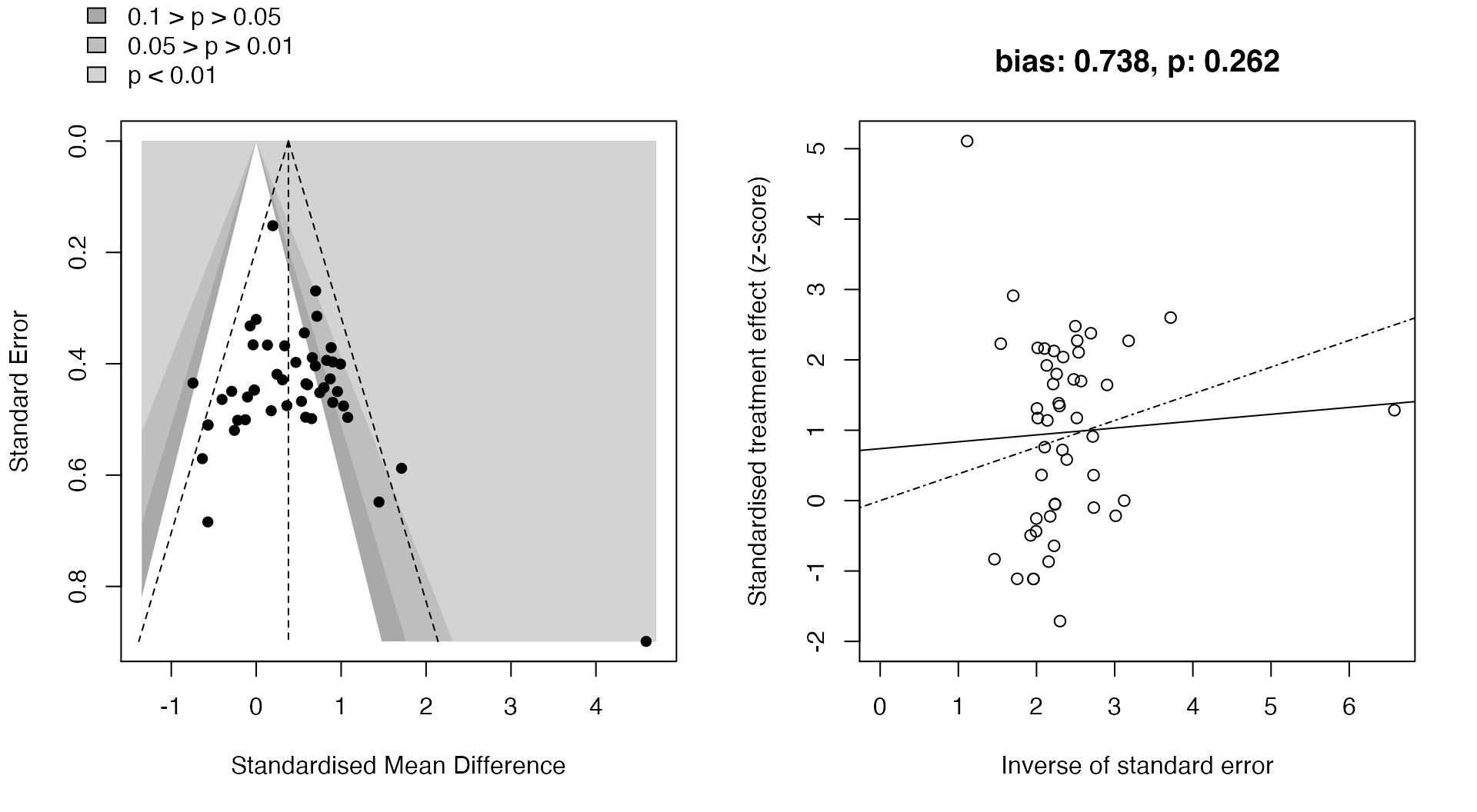
Small-study effects
Small-study effects (the phenomenon which smaller studies present different - often larger - treatment effects than bigger sample studies) may be visualized through contour-enhanced funnel plots, as well as through radial plots.
results$meta_analysis$Overall %>%
  plot_small_study_effects()
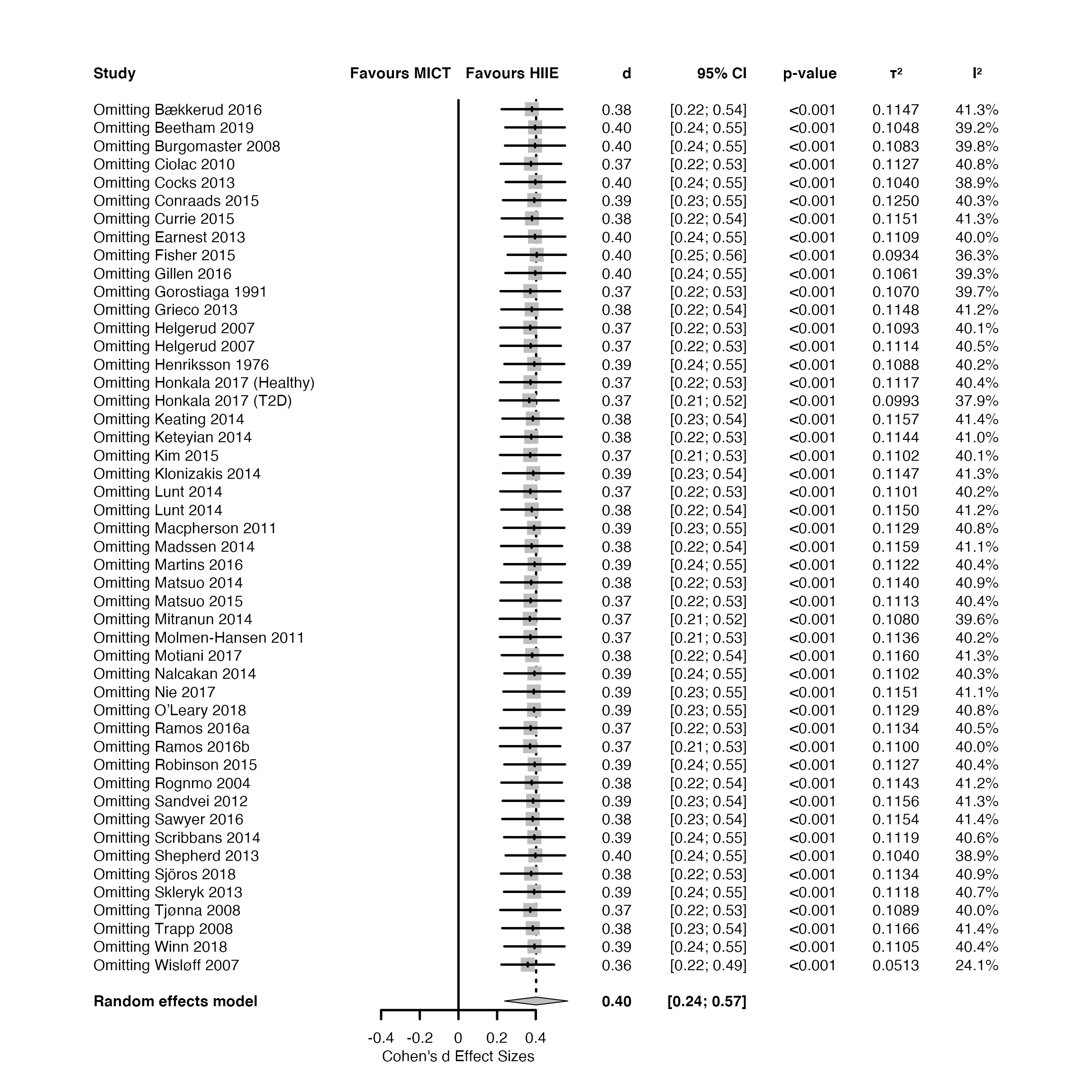
Sensitivity analysis
You may also access the results from the sensitivity analysis and produce a forest plot:
results$sensitivity_analysis$Overall
#>
#> Influential analysis (Random effects model)
#>
#>                                      SMD           95%-CI  p-value   tau^2     tau    I^2
#> Omitting Bækkerud 2016            0.3799 [0.2229; 0.5370] < 0.0001  0.1147  0.3387  41.3%
#> Omitting Beetham 2019             0.3963 [0.2424; 0.5503] < 0.0001  0.1048  0.3238  39.2%
#> Omitting Burgomaster 2008         0.3960 [0.2406; 0.5513] < 0.0001  0.1083  0.3290  39.8%
#> Omitting Ciolac 2010              0.3749 [0.2183; 0.5316] < 0.0001  0.1127  0.3357  40.8%
#> Omitting Cocks 2013               0.3979 [0.2440; 0.5518] < 0.0001  0.1040  0.3225  38.9%
#> Omitting Conraads 2015            0.3922 [0.2300; 0.5543] < 0.0001  0.1250  0.3536  40.3%
#> Omitting Currie 2015              0.3805 [0.2233; 0.5378] < 0.0001  0.1151  0.3393  41.3%
#> Omitting Earnest 2013             0.3959 [0.2390; 0.5527] < 0.0001  0.1109  0.3331  40.0%
#> Omitting Fisher 2015              0.4048 [0.2537; 0.5559] < 0.0001  0.0934  0.3057  36.3%
#> Omitting Gillen 2016              0.3973 [0.2426; 0.5520] < 0.0001  0.1061  0.3257  39.3%
#> Omitting Gorostiaga 1991          0.3718 [0.2175; 0.5262] < 0.0001  0.1070  0.3270  39.7%
#> Omitting Grieco 2013              0.3788 [0.2215; 0.5361] < 0.0001  0.1148  0.3388  41.2%
#> Omitting Helgerud 2007            0.3715 [0.2159; 0.5271] < 0.0001  0.1093  0.3307  40.1%
#> Omitting Helgerud 2007            0.3737 [0.2175; 0.5298] < 0.0001  0.1114  0.3338  40.5%
#> Omitting Henriksson 1976          0.3921 [0.2373; 0.5469] < 0.0001  0.1088  0.3298  40.2%
#> Omitting Honkala 2017 (Healthy)   0.3727 [0.2161; 0.5293] < 0.0001  0.1117  0.3342  40.4%
#> Omitting Honkala 2017 (T2D)       0.3660 [0.2138; 0.5182] < 0.0001  0.0993  0.3150  37.9%
#> Omitting Keating 2014             0.3848 [0.2272; 0.5424] < 0.0001  0.1157  0.3402  41.4%
#> Omitting Keteyian 2014            0.3767 [0.2192; 0.5341] < 0.0001  0.1144  0.3383  41.0%
#> Omitting Kim 2015                 0.3711 [0.2149; 0.5273] < 0.0001  0.1102  0.3319  40.1%
#> Omitting Klonizakis 2014          0.3869 [0.2298; 0.5440] < 0.0001  0.1147  0.3387  41.3%
#> Omitting Lunt 2014                0.3719 [0.2160; 0.5278] < 0.0001  0.1101  0.3318  40.2%
#> Omitting Lunt 2014                0.3791 [0.2218; 0.5365] < 0.0001  0.1150  0.3391  41.2%
#> Omitting Macpherson 2011          0.3911 [0.2344; 0.5479] < 0.0001  0.1129  0.3360  40.8%
#> Omitting Madssen 2014             0.3783 [0.2201; 0.5364] < 0.0001  0.1159  0.3405  41.1%
#> Omitting Martins 2016             0.3937 [0.2367; 0.5507] < 0.0001  0.1122  0.3350  40.4%
#> Omitting Matsuo 2014              0.3762 [0.2189; 0.5334] < 0.0001  0.1140  0.3376  40.9%
#> Omitting Matsuo 2015              0.3729 [0.2165; 0.5293] < 0.0001  0.1113  0.3337  40.4%
#> Omitting Mitranun 2014            0.3691 [0.2135; 0.5246] < 0.0001  0.1080  0.3287  39.6%
#> Omitting Molmen-Hansen 2011       0.3721 [0.2141; 0.5302] < 0.0001  0.1136  0.3371  40.2%
#> Omitting Motiani 2017             0.3814 [0.2235; 0.5392] < 0.0001  0.1160  0.3406  41.3%
#> Omitting Nalcakan 2014            0.3931 [0.2374; 0.5487] < 0.0001  0.1102  0.3320  40.3%
#> Omitting Nie 2017                 0.3896 [0.2318; 0.5473] < 0.0001  0.1151  0.3393  41.1%
#> Omitting O’Leary 2018             0.3911 [0.2344; 0.5478] < 0.0001  0.1129  0.3361  40.8%
#> Omitting Ramos 2016a              0.3732 [0.2156; 0.5308] < 0.0001  0.1134  0.3368  40.5%
#> Omitting Ramos 2016b              0.3705 [0.2142; 0.5268] < 0.0001  0.1100  0.3317  40.0%
#> Omitting Robinson 2015            0.3943 [0.2369; 0.5517] < 0.0001  0.1127  0.3358  40.4%
#> Omitting Rognmo 2004              0.3788 [0.2219; 0.5356] < 0.0001  0.1143  0.3381  41.2%
#> Omitting Sandvei 2012             0.3862 [0.2286; 0.5439] < 0.0001  0.1156  0.3400  41.3%
#> Omitting Sawyer 2016              0.3837 [0.2264; 0.5410] < 0.0001  0.1154  0.3397  41.4%
#> Omitting Scribbans 2014           0.3923 [0.2359; 0.5486] < 0.0001  0.1119  0.3344  40.6%
#> Omitting Shepherd 2013            0.3979 [0.2440; 0.5518] < 0.0001  0.1040  0.3225  38.9%
#> Omitting Sjöros 2018              0.3761 [0.2193; 0.5330] < 0.0001  0.1134  0.3367  40.9%
#> Omitting Skleryk 2013             0.3916 [0.2354; 0.5478] < 0.0001  0.1118  0.3344  40.7%
#> Omitting Tjønna 2008              0.3714 [0.2160; 0.5267] < 0.0001  0.1089  0.3300  40.0%
#> Omitting Trapp 2008               0.3845 [0.2263; 0.5427] < 0.0001  0.1166  0.3414  41.4%
#> Omitting Winn 2018                0.3930 [0.2372; 0.5488] < 0.0001  0.1105  0.3325  40.4%
#> Omitting Wisløff 2007             0.3585 [0.2220; 0.4950] < 0.0001  0.0513  0.2264  24.1%
#>
#> Pooled estimate                   0.4017 [0.2381; 0.5653] < 0.0001  0.1456  0.3816  47.1%
#>
#> Details on meta-analytical method:
#> - Inverse variance method
#> - DerSimonian-Laird estimator for tau^2
results$sensitivity_analysis$Overall %>%
  plot_metabolic()
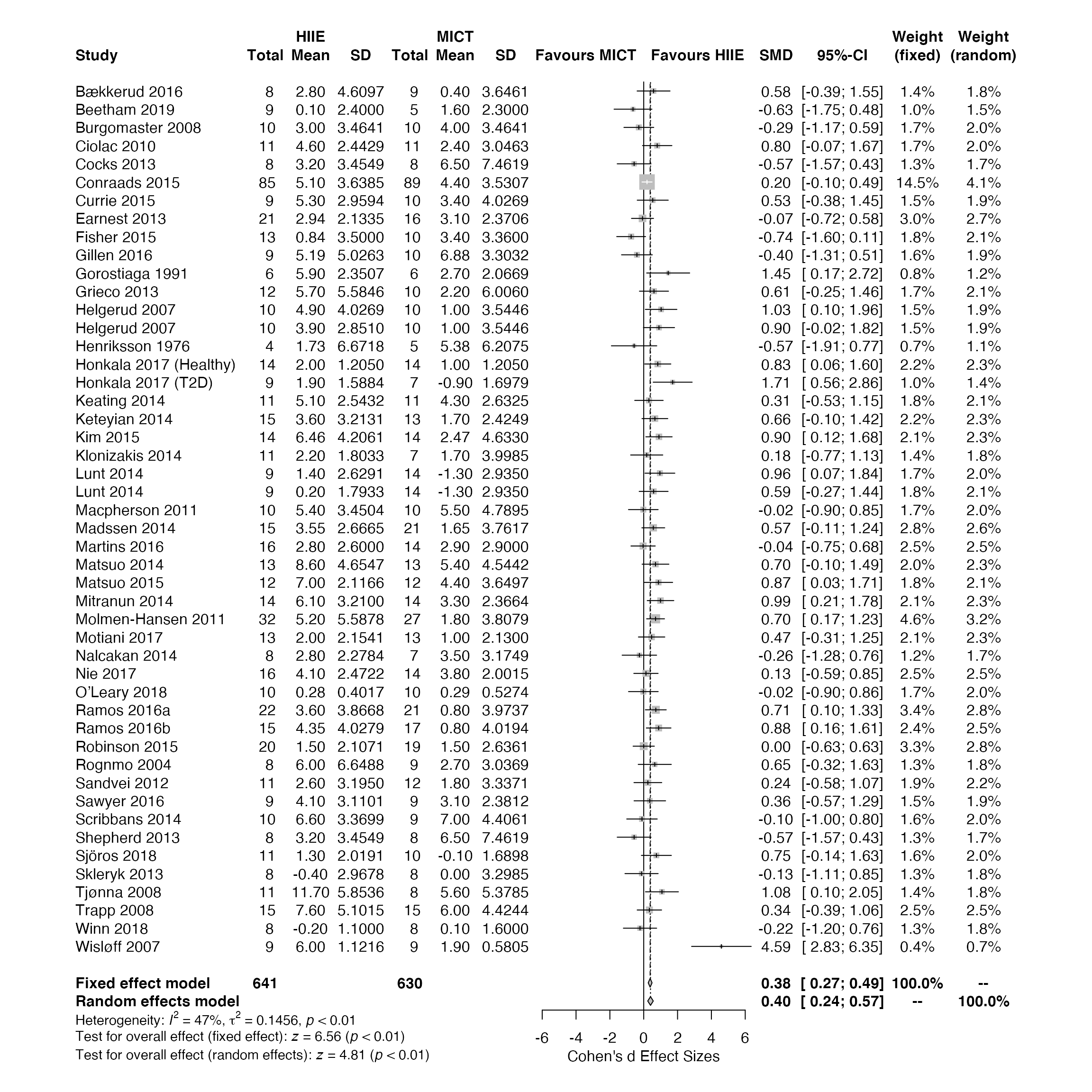
Overall meta-analysis
The overall meta-analysis results can be easily accessed through .$meta_analysis$Overall:
results$meta_analysis$Overall
#>                            SMD            95%-CI %W(fixed) %W(random)
#> Bækkerud 2016           0.5820 [-0.3903; 1.5542]       1.4        1.8
#> Beetham 2019           -0.6337 [-1.7518; 0.4845]       1.0        1.5
#> Burgomaster 2008       -0.2887 [-1.1698; 0.5924]       1.7        2.0
#> Ciolac 2010             0.7968 [-0.0715; 1.6650]       1.7        2.0
#> Cocks 2013             -0.5676 [-1.5671; 0.4320]       1.3        1.7
#> Conraads 2015           0.1953 [-0.1026; 0.4933]      14.5        4.1
#> Currie 2015             0.5330 [-0.3833; 1.4494]       1.5        1.9
#> Earnest 2013           -0.0715 [-0.7221; 0.5791]       3.0        2.7
#> Fisher 2015            -0.7440 [-1.5960; 0.1079]       1.8        2.1
#> Gillen 2016            -0.4021 [-1.3117; 0.5075]       1.6        1.9
#> Gorostiaga 1991         1.4458 [ 0.1749; 2.7166]       0.8        1.2
#> Grieco 2013             0.6057 [-0.2523; 1.4638]       1.7        2.1
#> Helgerud 2007           1.0281 [ 0.0955; 1.9607]       1.5        1.9
#> Helgerud 2007           0.9016 [-0.0184; 1.8216]       1.5        1.9
#> Henriksson 1976        -0.5694 [-1.9102; 0.7715]       0.7        1.1
#> Honkala 2017 (Healthy)  0.8299 [ 0.0579; 1.6019]       2.2        2.3
#> Honkala 2017 (T2D)      1.7112 [ 0.5592; 2.8633]       1.0        1.4
#> Keating 2014            0.3091 [-0.5316; 1.1498]       1.8        2.1
#> Keteyian 2014           0.6606 [-0.1020; 1.4232]       2.2        2.3
#> Kim 2015                0.9018 [ 0.1242; 1.6793]       2.1        2.3
#> Klonizakis 2014         0.1765 [-0.7729; 1.1259]       1.4        1.8
#> Lunt 2014               0.9567 [ 0.0748; 1.8385]       1.7        2.0
#> Lunt 2014               0.5858 [-0.2686; 1.4401]       1.8        2.1
#> Macpherson 2011        -0.0240 [-0.9005; 0.8526]       1.7        2.0
#> Madssen 2014            0.5664 [-0.1090; 1.2418]       2.8        2.6
#> Martins 2016           -0.0365 [-0.7538; 0.6809]       2.5        2.5
#> Matsuo 2014             0.6957 [-0.0960; 1.4874]       2.0        2.3
#> Matsuo 2015             0.8715 [ 0.0342; 1.7088]       1.8        2.1
#> Mitranun 2014           0.9929 [ 0.2078; 1.7781]       2.1        2.3
#> Molmen-Hansen 2011      0.6999 [ 0.1724; 1.2275]       4.6        3.2
#> Motiani 2017            0.4668 [-0.3123; 1.2460]       2.1        2.3
#> Nalcakan 2014          -0.2565 [-1.2750; 0.7620]       1.2        1.7
#> Nie 2017                0.1324 [-0.5857; 0.8505]       2.5        2.5
#> O’Leary 2018           -0.0213 [-0.8979; 0.8552]       1.7        2.0
#> Ramos 2016a             0.7144 [ 0.0977; 1.3311]       3.4        2.8
#> Ramos 2016b             0.8823 [ 0.1552; 1.6095]       2.4        2.5
#> Robinson 2015           0.0000 [-0.6279; 0.6279]       3.3        2.8
#> Rognmo 2004             0.6529 [-0.3245; 1.6302]       1.3        1.8
#> Sandvei 2012            0.2446 [-0.5765; 1.0658]       1.9        2.2
#> Sawyer 2016             0.3610 [-0.5704; 1.2925]       1.5        1.9
#> Scribbans 2014         -0.1028 [-1.0039; 0.7984]       1.6        2.0
#> Shepherd 2013          -0.5676 [-1.5671; 0.4320]       1.3        1.7
#> Sjöros 2018             0.7485 [-0.1373; 1.6343]       1.6        2.0
#> Skleryk 2013           -0.1275 [-1.1085; 0.8535]       1.3        1.8
#> Tjønna 2008             1.0772 [ 0.1042; 2.0502]       1.4        1.8
#> Trapp 2008              0.3351 [-0.3856; 1.0558]       2.5        2.5
#> Winn 2018              -0.2185 [-1.2014; 0.7644]       1.3        1.8
#> Wisløff 2007            4.5911 [ 2.8296; 6.3526]       0.4        0.7
#>
#> Number of studies combined: k = 48
#>
#>                         SMD           95%-CI    z  p-value
#> Fixed effect model   0.3794 [0.2661; 0.4927] 6.56 < 0.0001
#> Random effects model 0.4017 [0.2381; 0.5653] 4.81 < 0.0001
#>
#> Quantifying heterogeneity:
#>  tau^2 = 0.1456 [0.1246; 0.5265]; tau = 0.3816 [0.3529; 0.7256];
#>  I^2 = 47.1% [25.8%; 62.3%]; H = 1.38 [1.16; 1.63]
#>
#> Test of heterogeneity:
#>      Q d.f. p-value
#>  88.86   47  0.0002
#>
#> Details on meta-analytical method:
#> - Inverse variance method
#> - DerSimonian-Laird estimator for tau^2
#> - Jackson method for confidence interval of tau^2 and tau
#> - Cohen's d (standardised mean difference)
And the forest plot is generated through the generic function metabolic::plot_metabolic():
results$meta_analysis$Overall %>%
  plot_metabolic()
Subgroups meta-analysis
Overview
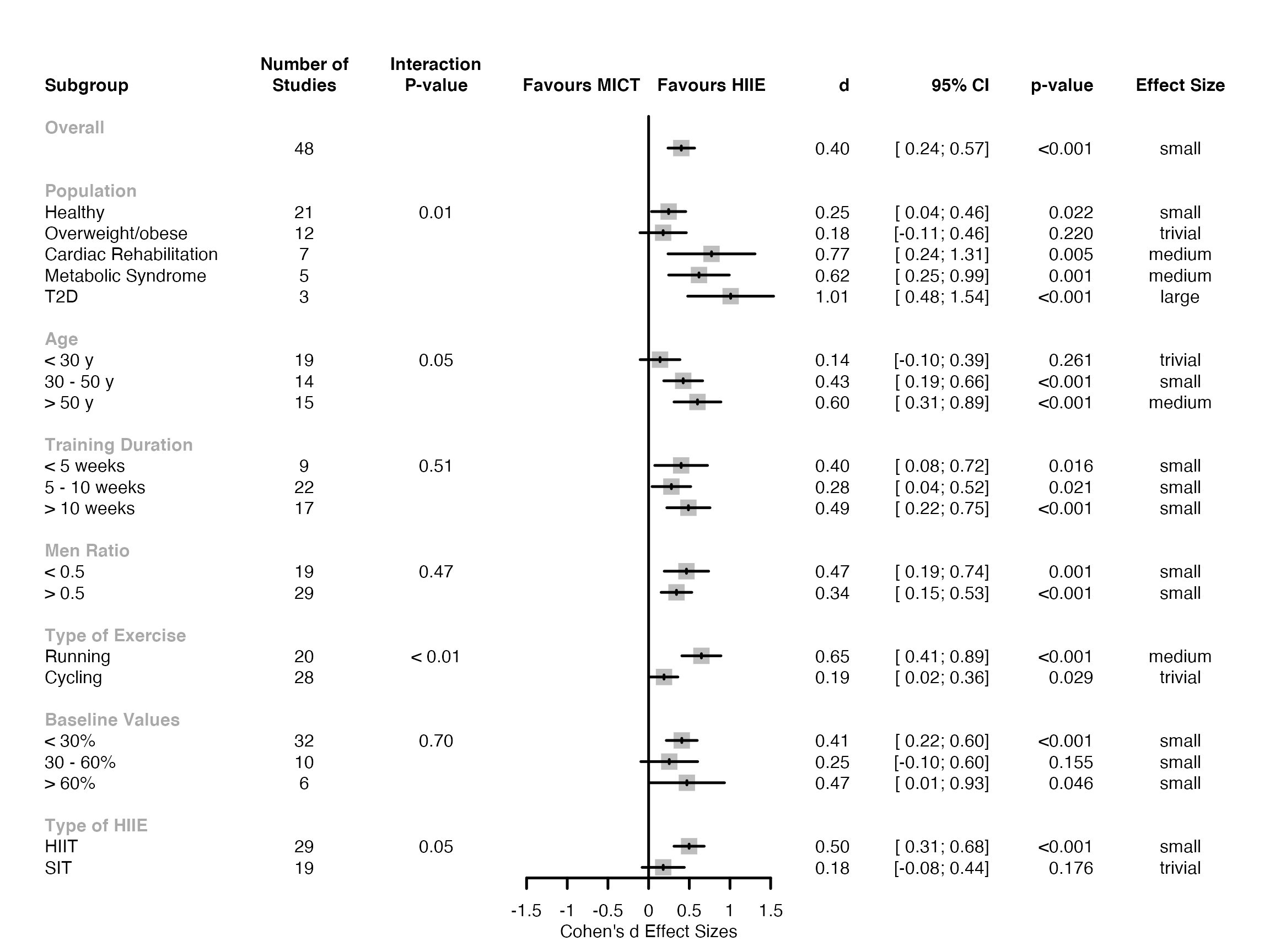
The overview of the subgroups meta-analysis results can be easily generated through the function metabolic::perform_bind()
results_bind <- perform_bind(results$meta_analysis)

results_bind
#>                           SMD            95%-CI     meta-analysis
#>                        0.4017 [ 0.2381; 0.5653]           Overall
#> Healthy                0.2461 [ 0.0354; 0.4568]        Population
#> Overweight/obese       0.1786 [-0.1067; 0.4640]        Population
#> Cardiac Rehabilitation 0.7734 [ 0.2385; 1.3082]        Population
#> Metabolic Syndrome     0.6192 [ 0.2461; 0.9922]        Population
#> T2D                    1.0085 [ 0.4805; 1.5365]        Population
#> < 30 y                 0.1405 [-0.1045; 0.3855]               Age
#> 30 - 50 y              0.4251 [ 0.1858; 0.6644]               Age
#> > 50 y                 0.6006 [ 0.3120; 0.8892]               Age
#> < 5 weeks              0.4000 [ 0.0756; 0.7244] Training Duration
#> 5 - 10 weeks           0.2799 [ 0.0420; 0.5178] Training Duration
#> > 10 weeks             0.4893 [ 0.2237; 0.7549] Training Duration
#> < 0.5                  0.4651 [ 0.1920; 0.7382]         Men Ratio
#> > 0.5                  0.3426 [ 0.1539; 0.5313]         Men Ratio
#> Running                0.6490 [ 0.4087; 0.8893]  Type of Exercise
#> Cycling                0.1894 [ 0.0189; 0.3598]  Type of Exercise
#> < 30%                  0.4076 [ 0.2175; 0.5977]   Baseline Values
#> 30 - 60%               0.2537 [-0.0956; 0.6030]   Baseline Values
#> > 60%                  0.4704 [ 0.0077; 0.9330]   Baseline Values
#> HIIT                   0.4978 [ 0.3119; 0.6837]      Type of HIIE
#> SIT                    0.1794 [-0.0802; 0.4390]      Type of HIIE
#>
#> Number of studies combined: k = 48
#>
#>                         SMD           95%-CI    z  p-value
#> Random effects model 0.4017 [0.2381; 0.5653] 4.81 < 0.0001
#>
#> Quantifying heterogeneity:
#>  tau^2 = 0.1456; tau = 0.3816; I^2 = 47.1% [25.8%; 62.3%]; H = 1.38 [1.16; 1.63]
#>
#> Test of heterogeneity:
#>      Q d.f. p-value
#>  88.86   47  0.0002
#>
#> Results for meta-analyses (random effects model):
#>                     k    SMD           95%-CI  tau^2    tau     Q   I^2
#> Overall            48 0.4017 [0.2381; 0.5653] 0.1456 0.3816 88.86 47.1%
#> Population         48 0.4017 [0.2381; 0.5653] 0.1456 0.3816 88.86 47.1%
#> Age                48 0.4017 [0.2381; 0.5653] 0.1456 0.3816 88.86 47.1%
#> Training Duration  48 0.4017 [0.2381; 0.5653] 0.1456 0.3816 88.86 47.1%
#> Men Ratio          48 0.4017 [0.2381; 0.5653] 0.1456 0.3816 88.86 47.1%
#> Type of Exercise   48 0.4017 [0.2381; 0.5653] 0.1456 0.3816 88.86 47.1%
#> Baseline Values    48 0.4017 [0.2381; 0.5653] 0.1456 0.3816 88.86 47.1%
#> Type of HIIE       48 0.4017 [0.2381; 0.5653] 0.1456 0.3816 88.86 47.1%
#>
#> Details on meta-analytical method:
#> - Inverse variance method
#> - DerSimonian-Laird estimator for tau^2
And the forest plot can be generated through the generic function metabolic::plot_metabolic():
results_bind %>%
  plot_metabolic()
Subgroups
Each subgroup analysis will have its own meta-analysis and meta-regression. Here is an example for the Population and Age subgroups:
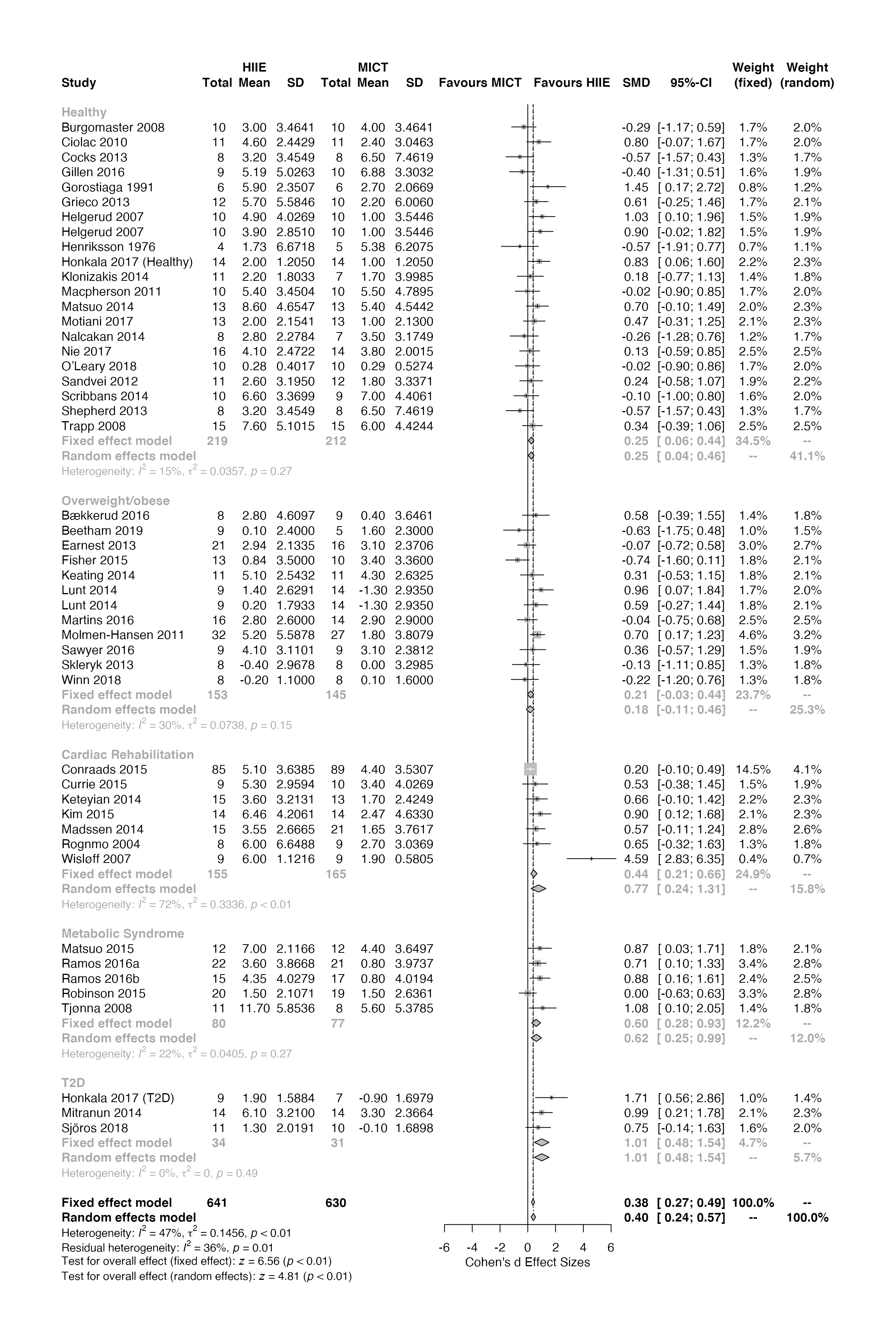
Population
results$meta_analysis$Population
#>                            SMD            95%-CI %W(fixed) %W(random)             population
#> Bækkerud 2016           0.5820 [-0.3903; 1.5542]       1.4        1.8       Overweight/obese
#> Beetham 2019           -0.6337 [-1.7518; 0.4845]       1.0        1.5       Overweight/obese
#> Burgomaster 2008       -0.2887 [-1.1698; 0.5924]       1.7        2.0                Healthy
#> Ciolac 2010             0.7968 [-0.0715; 1.6650]       1.7        2.0                Healthy
#> Cocks 2013             -0.5676 [-1.5671; 0.4320]       1.3        1.7                Healthy
#> Conraads 2015           0.1953 [-0.1026; 0.4933]      14.5        4.1 Cardiac Rehabilitation
#> Currie 2015             0.5330 [-0.3833; 1.4494]       1.5        1.9 Cardiac Rehabilitation
#> Earnest 2013           -0.0715 [-0.7221; 0.5791]       3.0        2.7       Overweight/obese
#> Fisher 2015            -0.7440 [-1.5960; 0.1079]       1.8        2.1       Overweight/obese
#> Gillen 2016            -0.4021 [-1.3117; 0.5075]       1.6        1.9                Healthy
#> Gorostiaga 1991         1.4458 [ 0.1749; 2.7166]       0.8        1.2                Healthy
#> Grieco 2013             0.6057 [-0.2523; 1.4638]       1.7        2.1                Healthy
#> Helgerud 2007           1.0281 [ 0.0955; 1.9607]       1.5        1.9                Healthy
#> Helgerud 2007           0.9016 [-0.0184; 1.8216]       1.5        1.9                Healthy
#> Henriksson 1976        -0.5694 [-1.9102; 0.7715]       0.7        1.1                Healthy
#> Honkala 2017 (Healthy)  0.8299 [ 0.0579; 1.6019]       2.2        2.3                Healthy
#> Honkala 2017 (T2D)      1.7112 [ 0.5592; 2.8633]       1.0        1.4                    T2D
#> Keating 2014            0.3091 [-0.5316; 1.1498]       1.8        2.1       Overweight/obese
#> Keteyian 2014           0.6606 [-0.1020; 1.4232]       2.2        2.3 Cardiac Rehabilitation
#> Kim 2015                0.9018 [ 0.1242; 1.6793]       2.1        2.3 Cardiac Rehabilitation
#> Klonizakis 2014         0.1765 [-0.7729; 1.1259]       1.4        1.8                Healthy
#> Lunt 2014               0.9567 [ 0.0748; 1.8385]       1.7        2.0       Overweight/obese
#> Lunt 2014               0.5858 [-0.2686; 1.4401]       1.8        2.1       Overweight/obese
#> Macpherson 2011        -0.0240 [-0.9005; 0.8526]       1.7        2.0                Healthy
#> Madssen 2014            0.5664 [-0.1090; 1.2418]       2.8        2.6 Cardiac Rehabilitation
#> Martins 2016           -0.0365 [-0.7538; 0.6809]       2.5        2.5       Overweight/obese
#> Matsuo 2014             0.6957 [-0.0960; 1.4874]       2.0        2.3                Healthy
#> Matsuo 2015             0.8715 [ 0.0342; 1.7088]       1.8        2.1     Metabolic Syndrome
#> Mitranun 2014           0.9929 [ 0.2078; 1.7781]       2.1        2.3                    T2D
#> Molmen-Hansen 2011      0.6999 [ 0.1724; 1.2275]       4.6        3.2       Overweight/obese
#> Motiani 2017            0.4668 [-0.3123; 1.2460]       2.1        2.3                Healthy
#> Nalcakan 2014          -0.2565 [-1.2750; 0.7620]       1.2        1.7                Healthy
#> Nie 2017                0.1324 [-0.5857; 0.8505]       2.5        2.5                Healthy
#> O’Leary 2018           -0.0213 [-0.8979; 0.8552]       1.7        2.0                Healthy
#> Ramos 2016a             0.7144 [ 0.0977; 1.3311]       3.4        2.8     Metabolic Syndrome
#> Ramos 2016b             0.8823 [ 0.1552; 1.6095]       2.4        2.5     Metabolic Syndrome
#> Robinson 2015           0.0000 [-0.6279; 0.6279]       3.3        2.8     Metabolic Syndrome
#> Rognmo 2004             0.6529 [-0.3245; 1.6302]       1.3        1.8 Cardiac Rehabilitation
#> Sandvei 2012            0.2446 [-0.5765; 1.0658]       1.9        2.2                Healthy
#> Sawyer 2016             0.3610 [-0.5704; 1.2925]       1.5        1.9       Overweight/obese
#> Scribbans 2014         -0.1028 [-1.0039; 0.7984]       1.6        2.0                Healthy
#> Shepherd 2013          -0.5676 [-1.5671; 0.4320]       1.3        1.7                Healthy
#> Sjöros 2018             0.7485 [-0.1373; 1.6343]       1.6        2.0                    T2D
#> Skleryk 2013           -0.1275 [-1.1085; 0.8535]       1.3        1.8       Overweight/obese
#> Tjønna 2008             1.0772 [ 0.1042; 2.0502]       1.4        1.8     Metabolic Syndrome
#> Trapp 2008              0.3351 [-0.3856; 1.0558]       2.5        2.5                Healthy
#> Winn 2018              -0.2185 [-1.2014; 0.7644]       1.3        1.8       Overweight/obese
#> Wisløff 2007            4.5911 [ 2.8296; 6.3526]       0.4        0.7 Cardiac Rehabilitation
#>
#> Number of studies combined: k = 48
#>
#>                         SMD           95%-CI    z  p-value
#> Fixed effect model   0.3794 [0.2661; 0.4927] 6.56 < 0.0001
#> Random effects model 0.4017 [0.2381; 0.5653] 4.81 < 0.0001
#>
#> Quantifying heterogeneity:
#>  tau^2 = 0.1456 [0.1246; 0.5265]; tau = 0.3816 [0.3529; 0.7256];
#>  I^2 = 47.1% [25.8%; 62.3%]; H = 1.38 [1.16; 1.63]
#>
#> Quantifying residual heterogeneity:
#>  I^2 = 36.0% [7.5%; 55.7%]; H = 1.25 [1.04; 1.50]
#>
#> Test of heterogeneity:
#>      Q d.f. p-value
#>  88.86   47  0.0002
#>
#> Results for subgroups (fixed effect model):
#>                          k    SMD            95%-CI     Q   I^2
#> Healthy                 21 0.2504 [ 0.0570; 0.4439] 23.47 14.8%
#> Overweight/obese        12 0.2063 [-0.0270; 0.4396] 15.67 29.8%
#> Cardiac Rehabilitation   7 0.4372 [ 0.2096; 0.6647] 21.47 72.1%
#> Metabolic Syndrome       5 0.6018 [ 0.2771; 0.9266]  5.15 22.3%
#> T2D                      3 1.0085 [ 0.4805; 1.5365]  1.44  0.0%
#>
#> Test for subgroup differences (fixed effect model):
#>                    Q d.f. p-value
#> Between groups 11.26    4  0.0238
#> Within groups  67.21   43  0.0105
#>
#> Results for subgroups (random effects model):
#>                          k    SMD            95%-CI  tau^2    tau
#> Healthy                 21 0.2461 [ 0.0354; 0.4568] 0.0357 0.1889
#> Overweight/obese        12 0.1786 [-0.1067; 0.4640] 0.0738 0.2717
#> Cardiac Rehabilitation   7 0.7734 [ 0.2385; 1.3082] 0.3336 0.5776
#> Metabolic Syndrome       5 0.6192 [ 0.2461; 0.9922] 0.0405 0.2012
#> T2D                      3 1.0085 [ 0.4805; 1.5365]      0      0
#>
#> Test for subgroup differences (random effects model):
#>                      Q d.f. p-value
#> Between groups   12.56    4  0.0136
#>
#> Details on meta-analytical method:
#> - Inverse variance method
#> - DerSimonian-Laird estimator for tau^2
#> - Jackson method for confidence interval of tau^2 and tau
#> - Cohen's d (standardised mean difference)
results$meta_analysis$Population %>%
  plot_metabolic()
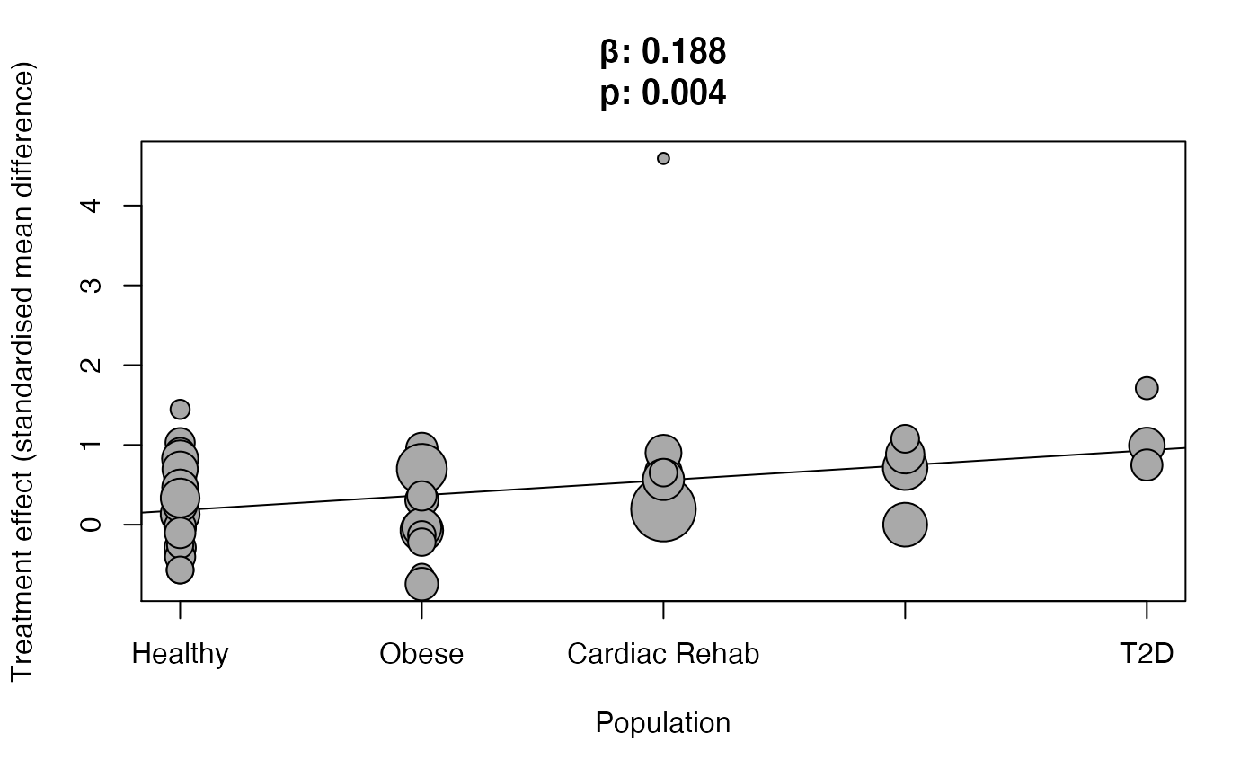
results$meta_regression$Population
#>
#> Mixed-Effects Model (k = 48; tau^2 estimator: DL)
#>
#> tau^2 (estimated amount of residual heterogeneity):     0.1359 (SE = 0.0690)
#> tau (square root of estimated tau^2 value):             0.3686
#> I^2 (residual heterogeneity / unaccounted variability): 43.71%
#> H^2 (unaccounted variability / sampling variability):   1.78
#> R^2 (amount of heterogeneity accounted for):            6.68%
#>
#> Test for Residual Heterogeneity:
#> QE(df = 43) = 76.3860, p-val = 0.0013
#>
#> Test of Moderators (coefficients 2:5):
#> QM(df = 4) = 10.8469, p-val = 0.0283
#>
#> Model Results:
#>
#>                               estimate      se     zval    pval    ci.lb   ci.ub
#> intrcpt                         0.2487  0.1283   1.9377  0.0527  -0.0029  0.5002  .
#> .byvarOverweight/obese         -0.0757  0.2077  -0.3645  0.7155  -0.4827  0.3313
#> .byvarCardiac Rehabilitation    0.4675  0.2426   1.9271  0.0540  -0.0080  0.9430  .
#> .byvarMetabolic Syndrome        0.4132  0.2692   1.5351  0.1248  -0.1144  0.9407
#> .byvarT2D                       0.8365  0.3683   2.2713  0.0231   0.1147  1.5583  *
#>
#> ---
#> Signif. codes:  0 '***' 0.001 '**' 0.01 '*' 0.05 '.' 0.1 ' ' 1
results$meta_regression$Population %>%
  plot_metabolic()
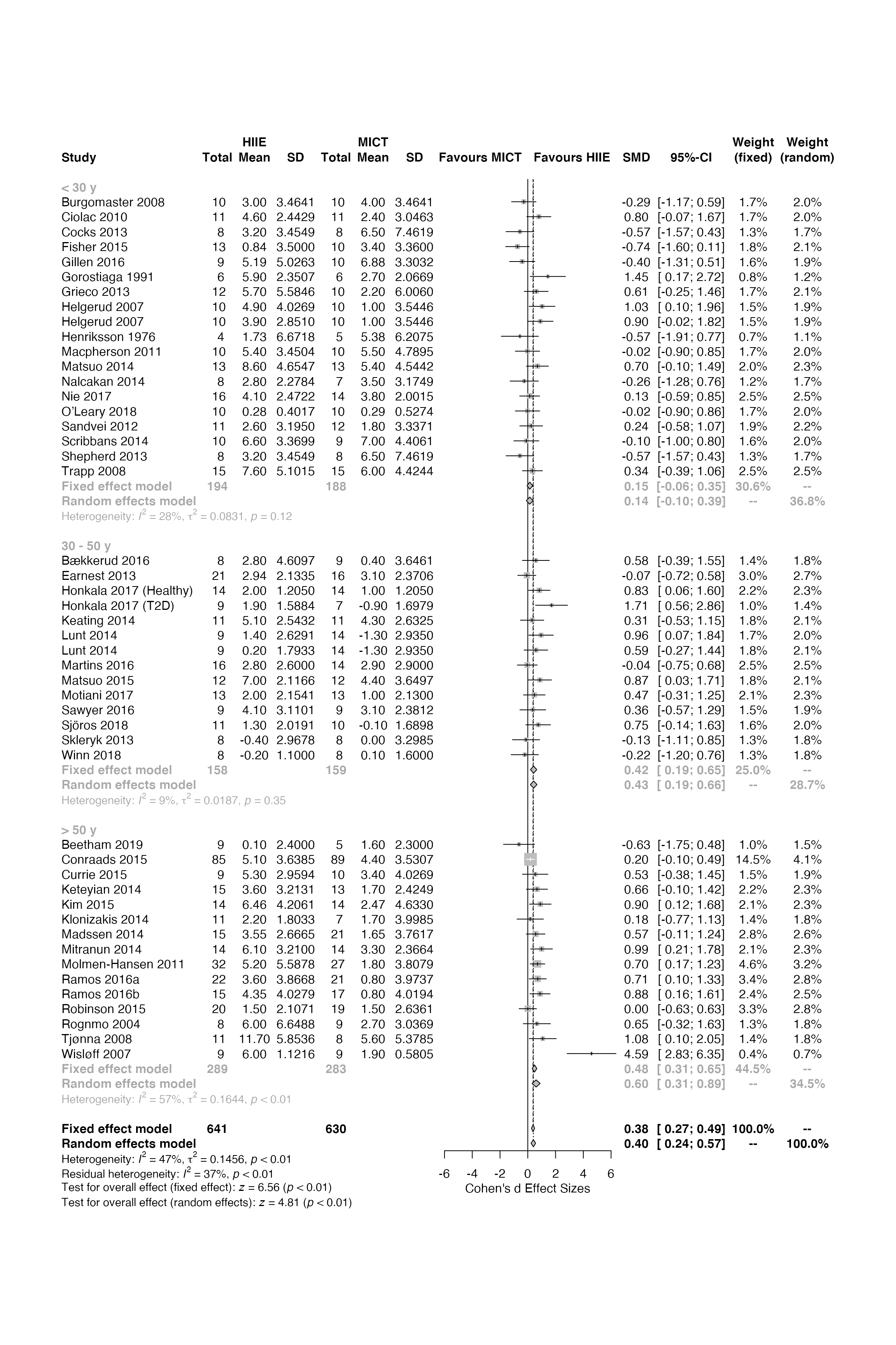
Age
results$meta_analysis$Age
#>                            SMD            95%-CI %W(fixed) %W(random) category_age
#> Bækkerud 2016           0.5820 [-0.3903; 1.5542]       1.4        1.8    30 - 50 y
#> Beetham 2019           -0.6337 [-1.7518; 0.4845]       1.0        1.5       > 50 y
#> Burgomaster 2008       -0.2887 [-1.1698; 0.5924]       1.7        2.0       < 30 y
#> Ciolac 2010             0.7968 [-0.0715; 1.6650]       1.7        2.0       < 30 y
#> Cocks 2013             -0.5676 [-1.5671; 0.4320]       1.3        1.7       < 30 y
#> Conraads 2015           0.1953 [-0.1026; 0.4933]      14.5        4.1       > 50 y
#> Currie 2015             0.5330 [-0.3833; 1.4494]       1.5        1.9       > 50 y
#> Earnest 2013           -0.0715 [-0.7221; 0.5791]       3.0        2.7    30 - 50 y
#> Fisher 2015            -0.7440 [-1.5960; 0.1079]       1.8        2.1       < 30 y
#> Gillen 2016            -0.4021 [-1.3117; 0.5075]       1.6        1.9       < 30 y
#> Gorostiaga 1991         1.4458 [ 0.1749; 2.7166]       0.8        1.2       < 30 y
#> Grieco 2013             0.6057 [-0.2523; 1.4638]       1.7        2.1       < 30 y
#> Helgerud 2007           1.0281 [ 0.0955; 1.9607]       1.5        1.9       < 30 y
#> Helgerud 2007           0.9016 [-0.0184; 1.8216]       1.5        1.9       < 30 y
#> Henriksson 1976        -0.5694 [-1.9102; 0.7715]       0.7        1.1       < 30 y
#> Honkala 2017 (Healthy)  0.8299 [ 0.0579; 1.6019]       2.2        2.3    30 - 50 y
#> Honkala 2017 (T2D)      1.7112 [ 0.5592; 2.8633]       1.0        1.4    30 - 50 y
#> Keating 2014            0.3091 [-0.5316; 1.1498]       1.8        2.1    30 - 50 y
#> Keteyian 2014           0.6606 [-0.1020; 1.4232]       2.2        2.3       > 50 y
#> Kim 2015                0.9018 [ 0.1242; 1.6793]       2.1        2.3       > 50 y
#> Klonizakis 2014         0.1765 [-0.7729; 1.1259]       1.4        1.8       > 50 y
#> Lunt 2014               0.9567 [ 0.0748; 1.8385]       1.7        2.0    30 - 50 y
#> Lunt 2014               0.5858 [-0.2686; 1.4401]       1.8        2.1    30 - 50 y
#> Macpherson 2011        -0.0240 [-0.9005; 0.8526]       1.7        2.0       < 30 y
#> Madssen 2014            0.5664 [-0.1090; 1.2418]       2.8        2.6       > 50 y
#> Martins 2016           -0.0365 [-0.7538; 0.6809]       2.5        2.5    30 - 50 y
#> Matsuo 2014             0.6957 [-0.0960; 1.4874]       2.0        2.3       < 30 y
#> Matsuo 2015             0.8715 [ 0.0342; 1.7088]       1.8        2.1    30 - 50 y
#> Mitranun 2014           0.9929 [ 0.2078; 1.7781]       2.1        2.3       > 50 y
#> Molmen-Hansen 2011      0.6999 [ 0.1724; 1.2275]       4.6        3.2       > 50 y
#> Motiani 2017            0.4668 [-0.3123; 1.2460]       2.1        2.3    30 - 50 y
#> Nalcakan 2014          -0.2565 [-1.2750; 0.7620]       1.2        1.7       < 30 y
#> Nie 2017                0.1324 [-0.5857; 0.8505]       2.5        2.5       < 30 y
#> O’Leary 2018           -0.0213 [-0.8979; 0.8552]       1.7        2.0       < 30 y
#> Ramos 2016a             0.7144 [ 0.0977; 1.3311]       3.4        2.8       > 50 y
#> Ramos 2016b             0.8823 [ 0.1552; 1.6095]       2.4        2.5       > 50 y
#> Robinson 2015           0.0000 [-0.6279; 0.6279]       3.3        2.8       > 50 y
#> Rognmo 2004             0.6529 [-0.3245; 1.6302]       1.3        1.8       > 50 y
#> Sandvei 2012            0.2446 [-0.5765; 1.0658]       1.9        2.2       < 30 y
#> Sawyer 2016             0.3610 [-0.5704; 1.2925]       1.5        1.9    30 - 50 y
#> Scribbans 2014         -0.1028 [-1.0039; 0.7984]       1.6        2.0       < 30 y
#> Shepherd 2013          -0.5676 [-1.5671; 0.4320]       1.3        1.7       < 30 y
#> Sjöros 2018             0.7485 [-0.1373; 1.6343]       1.6        2.0    30 - 50 y
#> Skleryk 2013           -0.1275 [-1.1085; 0.8535]       1.3        1.8    30 - 50 y
#> Tjønna 2008             1.0772 [ 0.1042; 2.0502]       1.4        1.8       > 50 y
#> Trapp 2008              0.3351 [-0.3856; 1.0558]       2.5        2.5       < 30 y
#> Winn 2018              -0.2185 [-1.2014; 0.7644]       1.3        1.8    30 - 50 y
#> Wisløff 2007            4.5911 [ 2.8296; 6.3526]       0.4        0.7       > 50 y
#>
#> Number of studies combined: k = 48
#>
#>                         SMD           95%-CI    z  p-value
#> Fixed effect model   0.3794 [0.2661; 0.4927] 6.56 < 0.0001
#> Random effects model 0.4017 [0.2381; 0.5653] 4.81 < 0.0001
#>
#> Quantifying heterogeneity:
#>  tau^2 = 0.1456 [0.1246; 0.5265]; tau = 0.3816 [0.3529; 0.7256];
#>  I^2 = 47.1% [25.8%; 62.3%]; H = 1.38 [1.16; 1.63]
#>
#> Quantifying residual heterogeneity:
#>  I^2 = 37.5% [10.5%; 56.3%]; H = 1.26 [1.06; 1.51]
#>
#> Test of heterogeneity:
#>      Q d.f. p-value
#>  88.86   47  0.0002
#>
#> Results for subgroups (fixed effect model):
#>             k    SMD            95%-CI     Q   I^2
#> < 30 y     19 0.1453 [-0.0602; 0.3509] 25.13 28.4%
#> 30 - 50 y  14 0.4194 [ 0.1920; 0.6469] 14.28  9.0%
#> > 50 y     15 0.4845 [ 0.3141; 0.6548] 32.56 57.0%
#>
#> Test for subgroup differences (fixed effect model):
#>                    Q d.f. p-value
#> Between groups  6.50    2  0.0388
#> Within groups  71.97   45  0.0065
#>
#> Results for subgroups (random effects model):
#>             k    SMD            95%-CI  tau^2    tau
#> < 30 y     19 0.1405 [-0.1045; 0.3855] 0.0831 0.2883
#> 30 - 50 y  14 0.4251 [ 0.1858; 0.6644] 0.0187 0.1369
#> > 50 y     15 0.6006 [ 0.3120; 0.8892] 0.1644 0.4054
#>
#> Test for subgroup differences (random effects model):
#>                     Q d.f. p-value
#> Between groups   6.03    2  0.0492
#>
#> Details on meta-analytical method:
#> - Inverse variance method
#> - DerSimonian-Laird estimator for tau^2
#> - Jackson method for confidence interval of tau^2 and tau
#> - Cohen's d (standardised mean difference)
results$meta_analysis$Age %>%
  plot_metabolic()
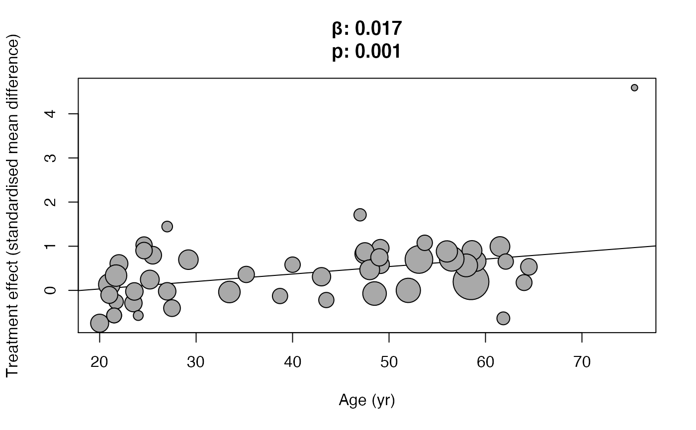
results$meta_regression$Age
#>
#> Mixed-Effects Model (k = 48; tau^2 estimator: DL)
#>
#> tau^2 (estimated amount of residual heterogeneity):     0.1149 (SE = 0.0614)
#> tau (square root of estimated tau^2 value):             0.3390
#> I^2 (residual heterogeneity / unaccounted variability): 40.88%
#> H^2 (unaccounted variability / sampling variability):   1.69
#> R^2 (amount of heterogeneity accounted for):            21.09%
#>
#> Test for Residual Heterogeneity:
#> QE(df = 46) = 77.8116, p-val = 0.0023
#>
#> Test of Moderators (coefficient 2):
#> QM(df = 1) = 10.6036, p-val = 0.0011
#>
#> Model Results:
#>
#>          estimate      se     zval    pval    ci.lb   ci.ub
#> intrcpt   -0.3055  0.2307  -1.3240  0.1855  -0.7576  0.1467
#> age        0.0169  0.0052   3.2563  0.0011   0.0067  0.0271  **
#>
#> ---
#> Signif. codes:  0 '***' 0.001 '**' 0.01 '*' 0.05 '.' 0.1 ' ' 1
results$meta_regression$Age %>%
  plot_metabolic()